Jupyter Notebook
Import the traveltime field and ray tracing class as well as numpy and matplotlib for data structures and plotting.
[1]:
from Anis_TTF_rays import ALI_FMM
import numpy as np
import matplotlib.pyplot as plt
import matplotlib

matplotlib.rc('text', usetex=True) # allows using latex for labels in plots
Define distance between points in grid and the source/reciever locations
[2]:
dnx = 1e-3
scx = dnx * np.array([1, 199])
scz = dnx * np.array([30, 180])
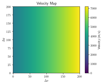
Create matrices for material properties. veln is the anisotropic orientation of the material, velpn is the material index of the material (by defalt material 1 is isotropic with velocity 1 if no materials are imput) and vel_map is a velocity scaling parameter (if using defalt materials these values are the velocity at each point. We create a velocity gradient from 3000 to 7200.
[3]:
veln = 0 * np.ones((201, 201))
velpn = 1 * np.ones((201, 201), dtype=int)
vel_map = np.zeros((201, 201))
for i in range(veln.shape[0]):
    for j in range(veln.shape[1]):
        vel_map[i, j] = 3000 + 21 * j
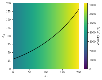
Plot of the velocity at each point in the grid.
[4]:
plt.imshow(vel_map, vmin=0)
plt.gca().invert_yaxis()
plt.colorbar(label="Velocity (m/s)")
plt.xlabel(r'$\Delta x$')
plt.ylabel(r'$\Delta y$')
plt.title("Velocity Map")
plt.show()
Initialise class without any materials as we are using isotropic materials.
[5]:
Forward_Model = ALI_FMM(veln, velpn, vel_map, scx, scz, dnx=1e-3)
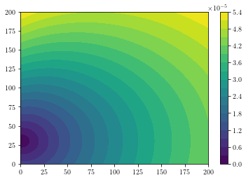
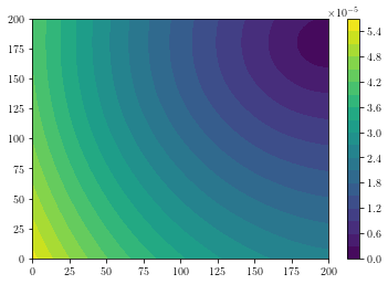
Traveltime Fields
Create traveltime fields and plot contour plots for each source location. The first time the traveltime fields are calculated will take longer than subsequent traveltime fields as files in folder \(\textrm{__pycache__}\) are created.
[6]:
Trav_TF = Forward_Model.update(veln, velpn, vel_map)
for i in range(2):
    plt.contourf(Trav_TF[i, :, :], 20)
    plt.colorbar()
    plt.show()

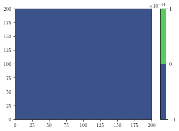
Create traveltime fields for only some of the sources. Sources not used return a matrix of zeros.
[7]:
Trav_TF_1 = Forward_Model.update(veln, velpn, vel_map, sources=np.array([0, 1]))

for i in range(2):
    plt.contourf(Trav_TF_1[i, :, :], 20)
    plt.colorbar()
    plt.show()
Ray Tracing
Create traveltime fields and perform ray tracing for all source/reciever pairs from material properties(each pair only finds one ray path i.e transducer is source or reciever). Times are returned as a matrix of traveltimes.
[8]:
trav_times = Forward_Model.find_all_TTF_rays(veln, velpn, vel_map)
print(trav_times)
[[0.00000000e+00 5.08845096e-05]
 [0.00000000e+00 0.00000000e+00]]
[9]:
ray_x, ray_y = Forward_Model.ray_path(0, 1)
plt.imshow(vel_map, vmin=0)
plt.gca().invert_yaxis()
plt.plot(ray_x, ray_y, "k")
plt.colorbar(label="Velocity (m/s)")
plt.xlabel(r'$\Delta x$')
plt.ylabel(r'$\Delta y$')
plt.show()
Defining materials using stiffness tensors
Define material properties using stifness tensors (in Pa) and density values (in Kg/\(\textrm{m}^3\)) for materials with stifness matrix in the form
Velocities in the y,z plane only dependant on stifness tensors \(c_{22}\), \(c_{23}\), \(c_{33}\), \(c_{44}\) and the density \(\sigma\).
[10]:
c_22 = 249.0e9
c_23 = 133.0e9
c_33 = 205.0e9
c_44 = 125.0e9
sigma = 7850

c_22 = 2.036e11
c_23 = 1.298e11
c_33 = 2.036e11
c_44 = 1.335e11
sigma = 7874
Define veln(anisotropic orientation), velpn(material index), vel_map(velocity scaling), transducer location and initialise class
[22]:
veln = 0 * np.ones((201, 201))
velpn = 1 * np.ones(veln.shape, dtype=int)
vel_map = 1 * np.ones(veln.shape)

scx = dnx * np.array([1, 199])
scz = dnx * np.array([100, 140])

Forward_Model_1 = ALI_FMM(veln, velpn, vel_map, scx, scz, dnx=1e-3)
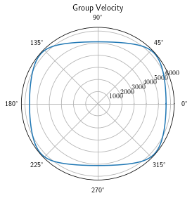
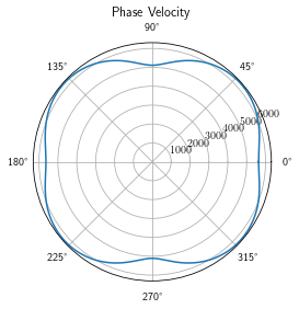
Plot group and phase velocity curves using stifness tensors and density. Two materials are then defined and added to defalt material. Defalt material(isotropic) has material index of 1 and two added materials have indices of 2 and 3.
[23]:
Forward_Model_1.generate_group_vel(c_22, c_23, c_33, c_44, sigma)
Forward_Model_1.generate_phase_vel(c_22, c_23, c_33, c_44, sigma)

materials = np.array([[c_22, c_23, c_33, c_44, 2 * sigma], [c_22, c_23, c_33, c_44, 3 * sigma]])
Forward_Model_1.add_materials(materials, True) # True used here to keep all previous materials
material id's of new materials are 2 - 3
All materials are removed(add True as second argument to keep previous materials) and new material is added(with material id of 1).
[24]:
Forward_Model_1.add_materials(np.array([c_22, c_23, c_33, c_44, sigma]))
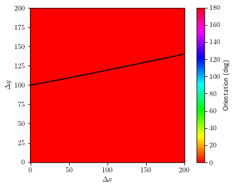
Transducer pairs are defined for ray tracing. Here the ray tracing is performed between one source reciever pair and so only one travel time field is calculated.
[25]:
trans = np.zeros((2, 2))
trans[1, 0] = 1
trans[0, 1] = 1
Calculate traveltime fields and ray paths for transducer pairs defined by trans and print ray path times.
[26]:
trav_times = Forward_Model_1.find_all_TTF_rays(veln, velpn, vel_map, trans_pairs=trans)
print(trav_times)
[[0.00000000e+00 3.54124066e-05]
 [3.54107926e-05 0.00000000e+00]]
[27]:
for i in range(trans.shape[0]):
    for j in range(trans.shape[0]):
        if trans[i, j] == 1:
            ray_x, ray_y = Forward_Model_1.ray_path(i, j)
            plt.imshow(veln, cmap="hsv", vmin=0, vmax=180)
            plt.gca().invert_yaxis()
            plt.plot(ray_x, ray_y, "k")
            plt.colorbar(label="Orientation (deg)")
            plt.xlabel(r'$\Delta x$')
            plt.ylabel(r'$\Delta y$')
            plt.show()

Solving christoffel equation during run time
Define material properties. Here we give a matrix for the material properties at each point in the grid with stifness tensors in MPa. Here the stiffness tensors must be defined as 64 bit integers. The christoffel equation will be solved during run time. The material index is set to 0 when using stiffness tensors and density (alows us to use a mixture of velocity curves and stifness tensors). velocity scaling (vel_map) set to 1 when using stifness tensors and density (velocitys can be scaled using density).
[17]:
c_22 = 249.0e9
c_23 = 133.0e9
c_33 = 205.0e9
c_44 = 125.0e9
sigma = 7850
stif_density = np.zeros((veln.shape[0], veln.shape[1], 5), dtype=np.int64)  # Stiffness tensors and density for all grid points in order c_22, c_23, c_33 and c_44
# Stiffness tensors in MPa due to 64bit limitations
stif_density[:, :, 0] = (c_22 / 1000000) * np.ones(veln.shape, dtype=np.int64)
stif_density[:, :, 1] = (c_23 / 1000000) * np.ones(veln.shape, dtype=np.int64)
stif_density[:, :, 2] = (c_33 / 1000000) * np.ones(veln.shape, dtype=np.int64)
stif_density[:, :, 3] = (c_44 / 1000000) * np.ones(veln.shape, dtype=np.int64)
stif_density[:, :, 4] = sigma * np.ones(veln.shape, dtype=np.int64)

veln = 20 * np.ones(veln.shape)
velpn = 0 * np.ones(veln.shape, dtype=int)
vel_map = 1 * np.ones(veln.shape)
Define transducer locations
[18]:
scx = dnx * np.array([1, 199, 100])
scz = dnx * np.array([100, 140, 1])
Initialise class using stifness tensors and density matrix
[19]:
Forward_Model_2 = ALI_FMM(veln, velpn, vel_map, scx, scz, stif_den=stif_density, dnx=1e-3)
Calculate traveltime field and ray paths.
[20]:
trav_times = Forward_Model_2.find_all_TTF_rays(veln, velpn, vel_map, stif_den=stif_density)
print(trav_times)
[[0.00000000e+00 3.56081540e-05 2.53646805e-05]
 [0.00000000e+00 0.00000000e+00 2.76255662e-05]
 [0.00000000e+00 0.00000000e+00 0.00000000e+00]]
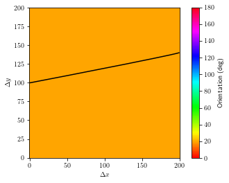
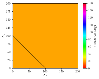
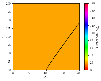
[21]:
for i in range(3):
    for j in range(3):
        if i < j:
            ray_x, ray_y = Forward_Model_2.ray_path(i, j)
            plt.imshow(veln, cmap="hsv", vmin=0, vmax=180)
            plt.gca().invert_yaxis()
            plt.plot(ray_x, ray_y, "k")
            plt.colorbar(label="Orientation (deg)")
            plt.xlabel(r'$\Delta x$')
            plt.ylabel(r'$\Delta y$')
            plt.show()